
Artificial Inteligence (AI) makes it possible to learn from experience in algorithmic, direct-forwarded way, adjust to new inputs and perform human-like tasks. Most AI examples that are heared about today – from chess-playing computers to self-driving cars – rely heavily on deep learning and natural language processing. One of the key AI tasks applied nowadays – image recognition and object detection.
Introduction
Neural Networks (NNs) are computational processing systems of which are heavily inspired by way biological nervous systems (such as the human brain) operate. NNs are mainly comprised of a high number of interconnected computational nodes (referred to as neurons), of which work entwine in a distributed fashion to collectively learn from the input in order to optimise its final output.
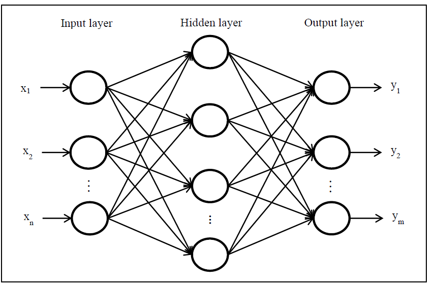
Fig. 1: A simple three layered feedforward neural network (FNN), comprised of a input layer, a hidden layer and an output layer
Convolutional Neureal Network
A Convolutional Neural Network (CNN) is a Deep Learning algorithm that can take in an input image, assign importance (learnable weights and biases) to various aspects/objects in the image, and be able to separate one from the other. The pre-processing required in a CNN is much lower as compared to other classification algorithms. While in primitive methods filters are hand-engineered, with enough training, CNNs have the ability to learn these filters/characteristics.
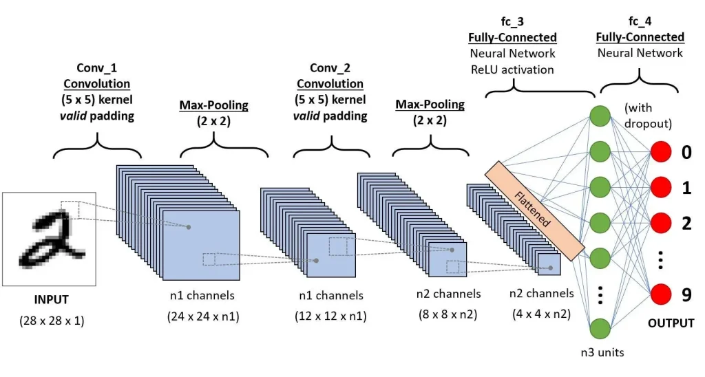
Fig. 2: A CNN general structure for classifying handwritten digits
Input image
As an input, CNN expects an RGB image that has been separated by its three color planes — Red, Green, and Blue. There are a number of such color spaces in which images exist — Grayscale, RGB, HSV, CMYK, etc.
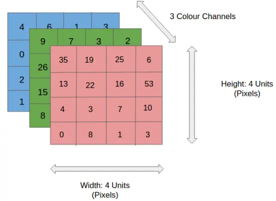
Fig. 3: Input image 4x4x3 RGB
Imagine how computationally intensive things would get once the images reach dimensions, say 8K (7680×4320). More pixels require more parameters to train. The role of CNN is to reduce the images into a form that is easier to process, without losing features that are critical for getting a good prediction. This is important to design an architecture that is not only good at learning features but also scalable to massive datasets. So, traditional NN works not with original image, but with smalled representation of image, with all important features presented.
CNN architecture
CNN architecture (Fig. 2) is typically composed of three types of layers (or building blocks): convolution, pooling, and fully connected layers, known as simple NN. When these layers are stacked, a CNN architecture has been formed.
Convolution layer
A convolution layer is a fundamental component of the CNN architecture that performs feature extraction, which typically consists of a combination of linear and nonlinear operations, i.e., convolution operation and activation function. The term convolution refers to the mathematical combination of two functions to produce a third function.
In the case of a CNN, the convolution is performed on the input data with the use of a filter or kernel (these terms are used interchangeably) to then produce a feature map. The filter moves to the right with a certain stride till it parses the complete width. Moving on, it hops down to the beginning (left) of the image with the same Stride and repeats the process until the entire image is traversed.
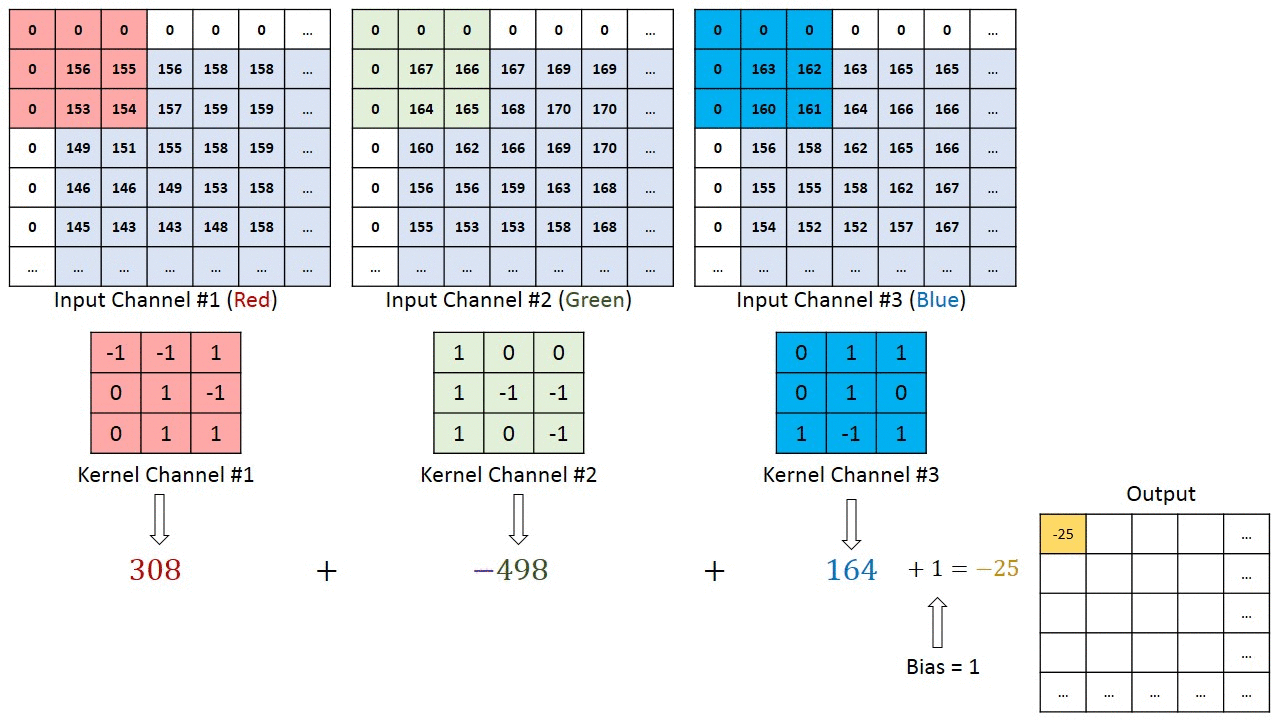
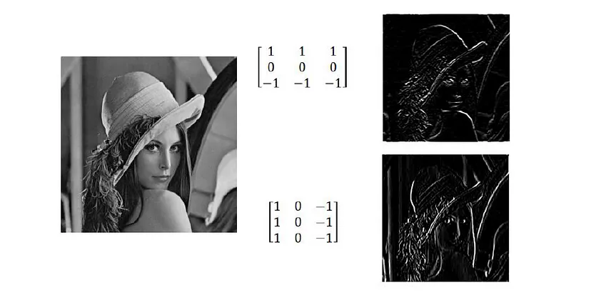
Fig. 5: Result of convolution for horizontal and vertical filters
Conventionally, the first Convolutional layer is responsible for capturing the low-level features such as edges, color, gradient orientation, etc. With added layers, the architecture adapts to the high-level features as well, giving a network that has a wholesome understanding of images in the dataset, similar to how we would.
As described later, the process of training a CNN model with regard to the convolution layer is to identify the kernels that work best for a given task based on a given training dataset. Kernels are the only parameters automatically learned during the training process in the convolution layer, on the other hand, the size of the kernels, number of kernels, padding, and stride are hyperparameters that need to be set before the training process starts.
Activation function
The outputs of a linear operation such as convolution are then passed through a nonlinear activation function. The most common nonlinear activation function used presently is the rectified linear unit (ReLU), which simply computes the function:
f(x) = max(0, x)
The reason, why other functions not used, like sigmoid or hyperbolic tangent (tanh) is simple: there are no pixel color representation for function output negative value. In general, ReLU just converts negative values to 0, while positive remains the same.
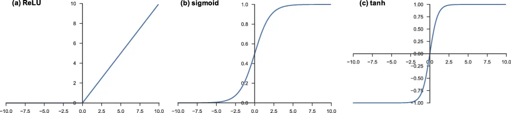
Fig. 6: Commonly applied activation functions – (a) rectified linear unit (ReLU), (b) sigmoid, and (c) hyperbolic tangent (tanh)
Pooling layer
A pooling layer provides a typical downsampling operation which reduces general image size, or, in other words, count of the feature maps in order to introduce a translation invariance to small shifts and distortions, and decrease the number of subsequent learnable parameters. It is important, that there is no learnable parameter in any of the pooling layers, whereas filter size, stride, and padding are hyperparameters in pooling operations, similar to convolution operations.
Max pooling
The most popular form of pooling operation is max pooling, which extracts patches from the input feature maps, outputs the maximum value in each patch, and discards all the other values (Fig. 7). A max pooling with a filter of size 2 × 2 with a stride of 2 is commonly used in practice. This downsamples the in-plane dimension of feature maps by a factor of 2.
Average pooling
Another commonly used pooling operation is a global average pooling. A global average pooling performs an extreme type of downsampling, where a feature map with size of height × width is downsampled into a 1 × 1 array by simply taking the average of all the elements in each feature map, whereas the depth of feature maps is retained. This operation is typically applied only once before the fully connected layers. The advantages of applying global average pooling are as follows: (1) reduces the number of learnable parameters, (2) enables the CNN to accept inputs of variable size and (3) noise suppression, but only in some certain cases, which are out of scope of this article.
Fully-connected layer
The fully-connected layer contains neurons of which are directly connected to the neurons in the two adjacent layers, without being connected to any layers within them. This is analogous to way that neurons are arranged in traditional forms of NN. (Fig 1)
Example: Building CNN for recognizing hand signs using MNIST dataset
Let’s try to use all knowledge base described before to build CNN for sign recognition. It is a well-known multi-class classification problem. We will be using the Sign Language MNIST dataset, which contains 28×28 images of hands depicting the 26 letters of the english alphabet. Please, fell free to check, look and investigate the original data.
Let’s get started!
Data preparations
At first, let’s import all required libs. We will be using NumPy + TensorFlow as a general NN framework. Also, let’s pick pyplot for data visualization.
import csv
import string
import numpy as np
import tensorflow as tf
import matplotlib.pyplot as plt
from tensorflow.keras.preprocessing.image import ImageDataGenerator, array_to_img
Download the training and test sets (the test set will actually be used as a validation set). If you have any problems, use direct link here
# sign_mnist_train.csv
!gdown --id 1z0DkA9BytlLxO1C0BAWzknLyQmZAp0HR
# sign_mnist_test.csv
!gdown --id 1z1BIj4qmri59GWBG4ivMNFtpZ4AXIbzg
Define some globals with the path to both files you just downloaded and look at how the data looks like within the csv file:
TRAINING_FILE = './sign_mnist_train.csv'
VALIDATION_FILE = './sign_mnist_test.csv'
with open(TRAINING_FILE) as training_file:
line = training_file.readline()
print(f"First line (header) looks like this:\n{line}")
line = training_file.readline()
print(f"Each subsequent line (data points) look like this:\n{line}")
As you can see, each file includes a header (the first line) and each subsequent data point is represented as a line that contains 785 values.
The first value is the label (the numeric representation of each letter) and the other 784 values are the value of each pixel of the image. Remember that the original images have a resolution of 28×28, which sums up to 784 pixels.
Parsing the dataset
Now let’s define function parse_data_from_input below.
This function should be able to read a file passed as input and return 2 numpy arrays, one containing the labels and one containing the 28×28 representation of each image within the file. These numpy arrays should have type float64.
def parse_data_from_input(filename):
"""
Parses the images and labels from a CSV file
Args:
filename (string): path to the CSV file
Returns:
images, labels: tuple of numpy arrays containing the images and labels
"""
# Use csv.reader, passing in the appropriate delimiter
# Remember that csv.reader can be iterated and returns one line in each iteration
arr = np.loadtxt(filename, delimiter=',', skiprows=1)
labels = np.transpose(arr[:,0])
images = arr[:, 1:].reshape((arr[:, 1:].shape[0], 28, 28))
return images, labels
# Test your function
training_images, training_labels = parse_data_from_input(TRAINING_FILE)
validation_images, validation_labels = parse_data_from_input(VALIDATION_FILE)
print(f"Training images has shape: {training_images.shape} and dtype: {training_images.dtype}")
print(f"Training labels has shape: {training_labels.shape} and dtype: {training_labels.dtype}")
print(f"Validation images has shape: {validation_images.shape} and dtype: {validation_images.dtype}")
print(f"Validation labels has shape: {validation_labels.shape} and dtype: {validation_labels.dtype}")
Expected Output:
Training images has shape: (27455, 28, 28) and dtype: float64
Training labels has shape: (27455,) and dtype: float64
Validation images has shape: (7172, 28, 28) and dtype: float64
Validation labels has shape: (7172,) and dtype: float64
Visualizing the numpy arrays
Now that you have converted the initial csv data into a format that is compatible with computer vision tasks, take a moment to actually see how the images of the dataset look like:
# Plot a sample of 10 images from the training set
def plot_categories(training_images, training_labels):
fig, axes = plt.subplots(1, 10, figsize=(16, 15))
axes = axes.flatten()
letters = list(string.ascii_lowercase)
for k in range(10):
img = training_images[k]
img = np.expand_dims(img, axis=-1)
img = array_to_img(img)
ax = axes[k]
ax.imshow(img, cmap="Greys_r")
ax.set_title(f"{letters[int(training_labels[k])]}")
ax.set_axis_off()
plt.tight_layout()
plt.show()
plot_categories(training_images, training_labels)
Creating the generators for the CNN
Now that it has successfully organized the data in a way that can be easily fed to Keras’ ImageDataGenerator, it is time for you to code the generators that will yield batches of images, both for training and validation. For this complete the train_val_generators function below.
Some important notes:
- The images in this dataset come in the same resolution so we don’t need to set a custom
target_sizein this case. In fact, you can’t even do so because this time you will not be using theflow_from_directorymethod (as in previous assignments). Instead you will use theflowmethod. - We need to add the “color” dimension to the numpy arrays that encode the images. These are black and white images, so this new dimension should have a size of 1 (instead of 3, which is used when dealing with colored images). Take a look at the function
np.expand_dimsfor this.
def train_val_generators(training_images, training_labels, validation_images, validation_labels):
"""
Creates the training and validation data generators
Args:
training_images (array): parsed images from the train CSV file
training_labels (array): parsed labels from the train CSV file
validation_images (array): parsed images from the test CSV file
validation_labels (array): parsed labels from the test CSV file
Returns:
train_generator, validation_generator - tuple containing the generators
"""
# In this section you will have to add another dimension to the data
# So, for example, if your array is (10000, 28, 28)
# You will need to make it (10000, 28, 28, 1)
# Hint: np.expand_dims
training_images = np.expand_dims(training_images, axis=3)
validation_images = np.expand_dims(validation_images, axis=3)
# Instantiate the ImageDataGenerator class
# Don't forget to normalize pixel values
# and set arguments to augment the images (if desired)
train_datagen = ImageDataGenerator(rescale = 1./255.,
rotation_range = 40,
width_shift_range = 0.2,
height_shift_range = 0.2,
shear_range = 0.2,
zoom_range = 0.2,
horizontal_flip = True)
# Pass in the appropriate arguments to the flow method
train_generator = train_datagen.flow(x=training_images,
y=tf.keras.utils.to_categorical(training_labels, num_classes=26),
batch_size=32)
# Instantiate the ImageDataGenerator class (don't forget to set the rescale argument)
# Remember that validation data should not be augmented
validation_datagen = ImageDataGenerator( rescale = 1.0/255. )
# Pass in the appropriate arguments to the flow method
validation_generator = validation_datagen.flow(x=validation_images,
y=tf.keras.utils.to_categorical(validation_labels, num_classes=26),
batch_size=32)
return train_generator, validation_generator
# Test your generators
train_generator, validation_generator = train_val_generators(training_images, training_labels,
 validation_images, validation_labels)
print(f"Images of training generator have shape: {train_generator.x.shape}")
print(f"Labels of training generator have shape: {train_generator.y.shape}")
print(f"Images of validation generator have shape: {validation_generator.x.shape}")
print(f"Labels of validation generator have shape: {validation_generator.y.shape}")
Expected Output:
Images of training generator have shape: (27455, 28, 28, 1)
Labels of training generator have shape: (27455,)
Images of validation generator have shape: (7172, 28, 28, 1)
Labels of validation generator have shape: (7172,)
Coding the CNN
One last step before training is to define the architecture of the model that will be trained.
Below provided create_model function. This function should return a Keras model that uses the Sequential or the Functional API. The last layer of this model should have a number of units that corresponds to the number of possible categories, as well as the correct activation function. Aside from defining the architecture of the model, you should also compile it so make sure to use a loss function that is suitable for multi-class classification.
It is better use no more than 2 Conv2D and 2 MaxPooling2D layers to achieve the desired performance. Feel free for your own experiments!
def create_model():
# Define the model
# Use no more than 2 Conv2D and 2 MaxPooling2D
model = tf.keras.models.Sequential([
# Note the input shape is the desired size of the image 150x150 with 3 bytes color
# This is the first convolution
tf.keras.layers.Conv2D(64, (3,3), activation='relu', input_shape=(28, 28, 1)),
tf.keras.layers.MaxPooling2D(2, 2),
# The second convolution
tf.keras.layers.Conv2D(64, (3,3), activation='relu'),
tf.keras.layers.MaxPooling2D(2,2),
# The third convolution
tf.keras.layers.Conv2D(128, (3,3), activation='relu'),
tf.keras.layers.MaxPooling2D(2,2),
# The fourth convolution
tf.keras.layers.Conv2D(128, (3,3), activation='relu'),
tf.keras.layers.MaxPooling2D(2,2),
# Flatten the results to feed into a DNN
tf.keras.layers.Flatten(),
# 512 neuron hidden layer
tf.keras.layers.Dense(512, activation='relu'),
tf.keras.layers.Dense(26, activation='softmax')
])
model.compile(optimizer = 'rmsprop',
loss = 'categorical_crossentropy',
metrics=['accuracy'])
### END CODE HERE
return model
# Save your model
model = create_model()
# Train your model
history = model.fit(train_generator,
epochs=15,
validation_data=validation_generator)
Now take a look at your training history:
# Plot the chart for accuracy and loss on both training and validation
acc = history.history['accuracy']
val_acc = history.history['val_accuracy']
loss = history.history['loss']
val_loss = history.history['val_loss']
epochs = range(len(acc))
plt.plot(epochs, acc, 'r', label='Training accuracy')
plt.plot(epochs, val_acc, 'b', label='Validation accuracy')
plt.title('Training and validation accuracy')
plt.legend()
plt.figure()
plt.plot(epochs, loss, 'r', label='Training Loss')
plt.plot(epochs, val_loss, 'b', label='Validation Loss')
plt.title('Training and validation loss')
plt.legend()
plt.show()
Note: All provided hyperparameteres for training were discovered using empirical research. Feel free to experiment with different NN layers, epochs number, activation function, filter size or count. Try to experiment with model’s architecture or the augmentation techniques to see if you can achieve higher levels of accuracy. A reasonable benchmark is to achieve over 99% accuracy for training and over 95% accuracy for validation within 15 epochs.
References
- Keiron O’Shea and Ryan Nash: An Introduction to Convolutional Neural Networks link.
- Niketh Narasimhan: Convolutional Neural Networks-An Intuitive approach link
- Rikiya Yamashita: Convolutional neural networks: an overview and application in radiology link
- Laurence Moroney and Andrew Ng: Convolutional Neural Networks in TensorFlow link
- Tim Dettmers: Understanding Convolution in Deep Learning link
- Sumit Saha: A Guide to Convolutional Neural Networks — the ELI5 way link